Planets around stellar remnants V, and summary

The final day of the Planets around stellar remnants conference included some of the more interesting, but also more speculative, talks. Andre Maeder opened with a general talk on life in the universe, concerning whose existence he takes a somewhat pessimistic view. There are many obstacles that stand in the way of the evolution of life, and complex life in particular. One of these is the problem of timescales: although it took only a few hundred million years for bacteria to develop on Earth, it took around 1.5 billion each for eukarya (complex single-celled organisms such as amoebae) and multicellular life to evolve. (Although, as pointed out by Lynn Rothschild in the discussion after the talk, complex life may have arisen earlier but left no trace in the fossil record, and in the lab multicellularity can be bred through artificial selection in just a few months.) By this arguement, a star must live for several billion years in order for complex life to develop. Since higher mass stars have shorter lifetimes, any star more massive than about 1.2 Solar masses would probably not have a long enough lifetime for complex life to develop. Similar arguments make the development of life in habitable zones around evolved stars, as described by William Danchi earlier in the week, less likely. Low mass M-dwarfs, although they live for a long time, are also unsuitable, since planets with an average temperature suitable for life are likely to be tidally locked, presenting one face permanently to the star, resulting in a planet with one parched and one frozen hemisphere. Other obstacles include perturbations from other planets in the system, volcanic and asteroidal hazards, the existence or not of plate tectonics, lack of water, or too much water. Most of these were debated after the talk or later in the day. Since we have a sample size of one known life-bearing planet to work from, any generalisation can be seen as somewhat hasty.

Lynn Rothschild then spoke about extremophiles: organisms that can survive extreme environmental conditions. The existence of such beings on Earth is a reminder that we should not take too anthropocentric a view when evaluating the prospects for another planet’s hosting life. “Extreme” is of course a relative term, and we ourselves tolerate levels of oxygen (a highly reactive chemical) that would be death to many microbes. The easiest environmental quality to measure astrophysically is a planet’s temperature, and while the traditional “habitable zone” around a star is the region which gives a planet a surface temperature that allows liquid water to exist, known species can actually survive at between -40 and 120 degrees celsius. The range for complex life is narrower, however, and many extremophiles (such as the tardigrade arthropods) are actually only “extremo-tolerant”: they can survive extremes such as dessication, but are only metabolically active in more comfortable environments.

Eric Agol next decribed the habitable zone around white dwarfs. This is located very close to the star, at around 0.01 AU. Although the WD cools as it ages, the cooling is sufficiently slow that the habitable zone can remain habitable for several billion years, so life may have ample time to evolve. Although such a planet would be tidally locked to the star, the extremely short spin period would induce atmospheric currents that could warm the night side, hence distributing heat more evenly over the planet’s surface. Such planets should be easy to detect: because the WD is so small, a planet a little larger than Earth could block out 100% of the star’s light, similar to a Solar eclipse by the Moon. Quite how such a planet would form is another question: it would have to have survived the star’s giant evolution, and then been moved close to the star at a later time.

Lisa Kaltenegger the described the habitability of exoplanets in more detail. The criterion that liquid water must exist on the planet’s surface means that the planet’s temperature as calculated simply from black-body absorption of the star’s light must be about -100 to 0 degrees celsius: it is raised above zero by a combination of clouds and the greenhouse effect. On Earth, these raise the average temperature from about -10 to +14. Proper modelling of exoplanets’ atmospheres must take into account geological and biological models as well as simple atmospheric chemistry: on Earth, the carbonate–silicate cycle driven by plate tectonics regulates the level of atmospheric CO2 and prevents the greenhouse effect from becoming too severe. The study of terrestrial planet atmospheres will be difficult, but not impossible, although targets close to the Sun will be required: the Earth-sized planets so far found by Kepler are all too distant.

Abel Méndez next attempted to quantify habitability. Instead of being a simple there-is-life/there-is-no-life dichotomy, he borrowed measures from ecology such as the Habitat Suitability Index that evaluate ecosystem productivity compared to some optimum. Another metric he proposed was an Earth Similarity Index, combining not just temperature but other planetary properties such as density to evaluate the similarity of a planet to Earth. There was some skepticism expressed as to how to calibrate such metrics, however.

Next, Yutaka Abe described modelling the habitability of dry planets: those with some water but not enough to form global oceans as on Earth (which he called “aqua planets”). On these planets, precipitation and evaporation are very local, so small wet regions can have very different conditions to dry ones. The liquid water habitable zone can then be much broader than for an aqua planet: such planets could have liquid water rather close to or distant from their star.

Marc Kuchner then talked about “carbon planets”, where carbon is more common than oxygen. The rocks on such planets would be carbides, rather than oxides and silicates as on Earth. The bulk composition of such planets could be inferred from spectroscopic observations of their atmospheres (cf the next talk). Such planets may not be uncommon, since the C/O ratios of stars are often greater than unity. And such planets could host life: as Marc said, “you don’t have to look very far to find organisms that metabolise carbon”. Although the biology of creatures on these planets could be rather different: instead of breathing an oxygen atmosphere and hunting carbon-rich food, the roles could be reversed, with carbon-breathing predators hunting smaller creatures for their valuable oxygen.

Finally, Nikku Madhusudhan described observations of WASP-12b, a transiting gas giant planet whose transmission spectrum can be modelled by a carbon-rich but oxygen-poor atmosphere. Although a giant planet, it shows that terrestrial carbon-rich planets may exist too.

This ended the contributed talks at the conference. Here is a list of what I personally felt to be the important and interesting topics raised over the week. In no particular order:

1. The statistics of planets around old and dead stars is still uncertain, due to the difficulty of detecting them. In particular, the first pulsar planets were discovered when only four or five millisecond pulsars were known, but now that hundreds are known there are still only a few planets. Did we just get lucky early on? See talks by Alex Wolszczan, Scott Ransom, and Bettina Posselt for Neutron Stars; Roberto Silvotti, Stephan Geier for subdwarfs; Matt Burleigh, Hans Zinnecker, JJ Hermes, Wei Wang for White Dwarfs; Andrzej Niedzielski, Johny Setiawan, Eva Villaver for subgiants and giants.
2. The existence of some planetary detections is strongly disputed, particularly those detected by the timing of stellar oscillations or eclipses of binaries. See talks by Richard Wade, JJ Hermes, and Steven Parsons, in particular. There is also a growing body of literature disputing some detections on grounds of dynamical stability (see here for the most recent example).
3. What happens when planets are engulfed by tides and their host stars’ expansion? (Eva Villaver, David Spiegel) Can they survive evaporation and the drag forces moving them into the stellar core? Can they unbind stellar envelopes to form subdwarf stars? (Stephane Charpinet, Stephane Greier)
4. How do planets form in the harsh environment around neutron stars? Are they captured from other systems (Steinn Sigurdsson), do they form in discs after supernova fallback or collision with another star (Brad Hansen), or are they the stirpped-down remnants of stars partially consumed by the neutron star (Sam Bates)? How can planets survive in the extreme radiation environment (Cole Miller), and could we detect discs around neutron stars (Geoff Bryden)?
5. There is now a growing consensus that the pollution of white dwarfs, and discs of dust and gas around them, are the result of planets or planetesimals being flung close to the star when planetary systems become unstable after the star becomes a white dwarf. John Debes and Shane Frewen modelled the delivery of particles to the star by planetary perturbations, and Kaitlin Kratter by binary perturbations, while Roman Rafikov modelled the evolution of the discs they form when tidally disrupted. How sensitive are such delivery mechanisms to the largely unknown architecture of extra-Solar planetary systems?
6. Despite the conditions for life to emerge and survive being very poorly known, the existance of a habitable zone where liquid water can survive for several hundred million years may be possible after a star has passed the red giant stage (William Danchi) and for several billion when a white dwarf (Eric Agol). Hence, searches for life around other planets should not be restricted only to Solar-type stars. The conditions for life to emerge and survive are highly uncertain, however, (Andre Maeder and Lynn Rothschild), and the chances of success of such a search are impossible to predict.

Thus ended a fruitful conference. Something I really liked was that, since Arecibo observatory is a radio-quiet zone, there was no wifi in the conference auditorium. That meant that all the audience had to pay attention to every single talk, instead of playing on their laptops. It’s no surprise then that the discussion sessions were among the most interactive I’ve ever seen. For those interested, the abstract booklet is available for download here, and the slides from the talks may be uploaded in future.

After the conference it was back on the plane to Madrid, via a scheduled stop, and unscheduled extra delay to fix the air conditioning, in the Dominican Republic. In the parched plain of Castilla I’ll not see anything so green again until my next holiday to the UK later this year.

Anisotropic frequency-dependent scattering of visible light from a G2V dwarf. Interesting fact: if you entitle a picture of a rainbow "rainbow.jpg", WordPress will censor it.

Planets around stellar remnants IV

Thursday’s sessions were largely devoted to theory and modelling rather than observations, and began with my new supervisor, Eva Villaver, reviewing various aspects of the effects of giant stars on any planets they host. Particularly during the Asymptotic Giant Branch, stellar radii attain very large values, of around 1AU for a star like the Sun. Tidal torques acting on the planet’s orbit, which are heavily dependent on the stellar radius, are therefore very strong, and any Jovian planet within about 3AU of a Solar-mass star will be engulfed. What happens then is a difficult question. Although we heard talks earlier in the week about the potential of planets to unbind stellar envelopes to form hot subdwarfs, this may not be possible for planets less than 10 Jovian masses or so. Planets may also be evaporated by the high energy flux, losing about 1 Jovian mass of matter every million years. The prospects for planets surviving from the main sequence to the white dwarf phase seem bleak.

Harold Yorke then discussed planet formation around massive O stars. The discs surrounding these stars when young are very massive but very short-lived, so planet formation by core accretion–colliding dust grains and rocks to slowly build up planets–is not likely, but planet formation by gravitational instabilities in the gas disc is possible. However, the final mass of these `planets’ is uncertain, as they would accrete a great deal of material in the massive gas disc, and may well end up as small stars.

Kaitlin Kratter then discussed the stability of planets in orbits around one component of a binary system, as the stars evolve and lose mass. The regions where orbits are stable on the main sequence change when a star in a binary system loses mass, and previously stable planets can be captured into orbits around the other star, or collide with one of the stars. This may provide another way of delivering material to polluted white dwarfs, although few polluted WDs are known to have binary companions.

Dimitri Veras next described how the orbits of circumbinary planets–in which the planet orbits both stars of a binary system–change under stellar evolution. Here the orbit of the planet expands as mass is lost from the binary system, and if mass loss is very rapid the planet can be expelled from the system entirely. Planets around binaries of stars of one to two Solar masses are however usually safe, unless they orbit at very large distances.

Stein Sigurdsson then talked about the planet orbiting the binary pulsar PSR 1620-26, in the globular cluster M4. Due to the high stellar densities in globular clusters, capture of a planet from another star is a possible explanation for the planet’s origin. However, planets are not found around main sequence stars in globular clusters, so the origin may still be a puzzle.

Eduardo Martín presented a novel mechanism for creating Hot Jupiter planets, on orbits very close to their host stars. Rather than forming in the primordial circumstellar disc, he proposed that they arise from a merger of a contact binary (W UMa star), during which a fresh disc of material is thrown out. This may offer an explanation for the large radii of the so-called inflated hot Jupiters.

Roman Rafikov discussed models for the evolution of discs around WDs. Following the disruption of an asteroid, the material must be brought in from a disc at around a Solar radius to the surface of the White Dwarf, in order to cause observed metal pollution. The nature of a dust disc is similar to Saturn’s rings, and the timescale for such rings to spread is very long: Saturn has not accreted its ring material despite having several Gyr in which to do so. However, around WDs, two effects enhance the movement of dust towards the star. One is the Poynting–Robertson effect, a drag force caused by the starlight. The other is gas drag from dust that gets close to the WD and sublimates. This latter effect can trigger rapid bursts of accretion which can move significant quantities of material onto the WD quickly.

Noam Soker discussed transient events arising from the destruction of planets and planetesimals. Such events can be very violent, with the merger of a Brwon Dwarf and a Jovian planet for example casuing the BD to brighten by up to 8 magnitudes, and the destruction of an asteroid by a neutron star offering an explanation for an unusual gamma ray burst in 2010.

Shane Frewen then presented work on the dynamics of planetesimals perturbed by eccentric planets, attempting to explain how to scatter asteroids close to a White Dwarf in order to provide metal pollution. The most effective planets for sending bodies close to the star are highly eccentric and of mass somewhat less than Jupiter’s. However, many planetesimals orbiting close to planets are destabilised on the main sequence, and after the star loses mass on its way to beoming a white dwarf not many more planetesimals are destabilised. A larger source population could however be provided if the planetesimals experience gas drag in the planetary nebula, and migrate in to the previously depopulated region.

Brad Hansen described models of the formation of rocky planets around pulsars. The idea is to integrate the orbits of a collection of large protoplanets, assumed to have formed from a disc, in the same way as is done for terrestrial planet formation around Solar type stars. A variety of protoplanet configurations, corresponding to the discs expected from different formation mechanisms, such as supernova fallback and WD merger, were tried. The configuration yielding the configuration most like the planets of PSR B1257+12 corresponded to a supernova fallback disc, although since these may not be rare this raises the question of why there are not many more pulsar planets.

To end Thursday’s talks, Cole Miller gave a grimmer assessment of the prospects for forming planets around pulsars, since the environment in which they form is so harsh: heating from the pulsar’s radiation and ablation by the wind could easily destroy planetesimals of up to a kilometer in size. This suggests that planets must have formed quickly, and the planet formation process would be all-or-nothing: there could be no asteroid belts surviving as in main sequence planetary systems such as our own.

After Thursday’s talks, the conference dinner took place, in a seaside restaurant with views of the old Arecibo lighthouse:

Late 19th Century Arecibo lighthouse. The rocks in the water around here looked pretty vicious.

Planets around stellar remnants III

Wednesday saw a crammed schedule of talks. We first moved away from planets to dusty discs around stellar remnants, with Geoff Bryden opening with a review of dust discs around Main Sequence stars, and then a description of the different physical processes influencing dust discs around Neutron Stars. Notably, pulsar winds can ablate dust grains and significantly alter the size distribution of particles. There is at least one neutron star with a dust disc: 4U 2259+586, an anomalous X-ray pulsar (these pulsars are not accreting gas; the X-rays come from magnetospheric processes) which has mid IR emission from dust but no sign of gas.

Next, Ben Zuckerman reviewed the study of White Dwarf pollution. Due to the very strong gravitational fields of WDs, any metals in their atmospheres sink on a timescale of years to megayears depending  on atomic mass, so any metals present in their atmosphere must have been delivered at astronomically recent times. The best candidate for the pollution is asteroids which are tidally disrupted when they pass close to the WD, and then are accreted onto it. Indeed, for the polluted WDs whose metal content is known in detail, the composition of the pollution is very similar to the composition of rocky bodies in the inner Solar System. At least 25% of WDs show pollution, suggesting that bombardment of them by asteroids is common. Ben closed with an intriguing peek at an upcoming result showing that a dust disc around a Main Sequence star appears to have disappeared in 2009/10…

Next John Debes described the sizes of these WD dust discs in more vivid terms: roughly, they are similar in size to Saturn’s rings, and vary from thin belts to very wide discs. John then described how asteroids in a Solar-System type asteroid belt can be destabilised by a Jovian planet as the star loses mass just before becoming a WD–the Kirkwood gaps in the asteroid belt where orbits are unstable grow and more asteroids are encompassed by the unstable region. A few per cent of the unstable asteroids get hurled onto orbits that take them sufficicently close to the WD to be tidally disrupted and form a disc and provide a pollution source.

Jay Farihi next gave more physical details about the dust in these discs. They typically show evidence for silicate rocks in their infrared spectra, suggesting an origin from terrestrial planets or asteroids. Estimated disc masses are around the size of large asteroids in the Solar System, as are the estimated masses of accreted material providing the atmospheric pollution. Together, these talks gave a very strong case for the idea that WD pollution and dust discs are caused by asteroids passing close to the WD.

Next, Boris Gaensicke described how some WDs have gaseous discs. These can be hydrogen dominated, but several are only composed of gaseous metals. The gas emission lines are split, allowing the Keplerian velocity of the gas to be determined. Several show time variability, hinting at non-circular discs. Furthermore, the emission lines can be highly asymmetric, which is naturally explained as us seeing a tidal stream from a recent disruption event.

Stephan Hartmann then described explicitly the modelling of asymmetric gaseous emission lines towards the WD SDSS J1228+1040, where a simple viscous disc model can reproduce the observations. Such a model is however unrealistic as it ignores illumination from the WD, actually the dominant source of heating.

Patrick Dufour then described another particular WD, SDSS J0738+1835, which has accreted a body at least as big as Ceres, the largest asteroid, and also hosts a disc with gas and dust components. The elemental composition of the accreted matter is rather deficient in refractories, in comparison to most other polluted WDs, so the composition of extra-Solar asteroids and planets is clearly somewhat variable between systems.

Kate Su and Jana Bilikova then teamed up to talk about dust discs around hot, young WDs stil surrounded by planetary nebulae. Spitzer has found discs around 9 such WDs, well inside the large planetary nebula, a typical example being the WD and disc at the centre of the Helix Nebula. 6 of the discs are similar to the Helix disc, explicable as Kuiper Belt type discs that have survived the star’s giant stages and mass loss. The other three are more complicated, as there appears to be a close binary companion to the WD in each case, as well as the disc.

We then moved back to planets, Andrzej Niedzielski talking about planets around sub-giant and giant stars. Several dozen of these are now known, with none having been found within about 0.5 AU of the host star, in contrast to planets around Main Sequence stars where many are on close orbits. It is not clear whether this is the result of tidal engulfment of the close-in planets, or a signpost of the formation of the planets, since the masses of the giants targetted tend to be higher than the masses of the main sequence stars. He also pointed out that some giant stars have far more Lithium than they should. Lithium is quickly destroyed inside stars and should not persist until the giant stages, so perhaps these stars have had their lithium replenished by swallowing a planet or two.

Johny Setiawan then described some giant stars and their planets in some detail. Many of these giants are of very low metalicity, somewhat challenging for conventional theories of planet formation. He also showed an RV curve for a 20 Solar mass O-type star, hinting at a substellar companion. If confirmed, this will be the most massive host of an exoplanet or low-mass brown dwarf known.

David Spiegel next talked about the survival of planets to tidal forces as stars expand, and what happens if they get engulfed by the expanding stellar envelope. The huge uncertainties in tidal theory make it very hard to predict a planet at a radius of a few AU will survive its host’s expansion or not. It is also hard to produce planets that end up on intermediate orbits of a few tenths of an AU, or low mass planets on any orbit less than about 1AU, with our current understanding of what happens to planets that enter the envelope. Yet, these objects are seen.

Frederic Hessman finished the day with a description of the three circumbinary planets discovered by Kepler (two in this week’s Nature). He then described the previously reported circumbinary planets detected by timing the eclipses of the binary, drawing attention to many problems in the analyses. These include varying eclipse durations as well as times (not expected from planetary perturbations), inconsistency in the dyanical models (typically the influence of the binary on the putative planet’s orbit is neglected, so the solution is not self-consistent), to trivial dynamical instability (a notorious example, to which already at least two refutation papers have been published, actually claims two planets whose orbits overlap…). He made an explicit call for “stricter referees”. Of the 10 or so timing-based circumbinary planet claims, only NN Serpentis looks robust.

Planets around stellar remnants II

The morning of the second day was dedicated to planets orbiting white dwarfs (WDs). Matt Burleigh opened with an overview of recent attempts to detect substellar objects around WDs with direct imaging. So far there are few positive results, with the UKIDSS survey having turned up a few candidates, showing maybe a half of a per cent of white dwarfs host wide L/T dwarf companions, and a possible Y dwarf companion to GJ3483 in a very wide (~2500 AU) orbit. Meanwhile, constraints from the DODO survey show that <5% of WDs host companions heavier than 13 Jovian masses on orbits between about 10 and 60 AU, and less than a third host such companions heavier than 6 Jovian masses. A great number of such companions is perhaps not to be expected, given that they are not seen around many main sequence stars.

Hans Zinnecker then gave another negative result, from a small NICMOS survey of 7 Hyades WDs, none of them having companions heavier than 10 Jovian masses. WDs in cludters are very useful to study, since their total age can be determined with reasonable accuracy, and the age is needed to convert a brown dwarf flux into an actual mass.

JJ Holmes then talked about the use of the timing of WD oscillation modes to detect planets. Periodic signals that could arise from acceleration due to planets have been observed from several pulsating WDs. Among them is GD66 (aka V361 Aurigae), where a planet on a ~6 year orbit was announced in 2007. Since then, another “orbital” cycle has been observed, which would seem to strengthen the attribution of the signal to a planet rather than some quasi-periodic effect. However, when the timing variations of a separate mode were analysed, it was found to vary with the same period but exactly the opposite phase. Hence, the changes cannot be due to the acceleration of the whole star due to the planet, and the signals must be due to some as-yet unidentified asteroseismological mechanism. This underlines the importance of confirming “planetary” signals from timing analysis with independent measurements.

Wei Wang next presented evidence for the existence of a brown dwarf or low-mass red dwarf orbiting the young WD at the centre of the planetary nebula NGC 246. A radial velocity signal with a period of 4 days and amplitude of ~9 km/s was seen, which could be due to an object of mass at least 60 times Jovian. There also appears to be a an IR excess, indicative of hot dust or a companion radiating in the infrared. There was some criticism from the audience, since planetary nebulae are very confusing environments and contamination of the spectra could be a serious issue.

To end tuesday morning’s talks, Steven Parsons discussed the detection of companions by timing eclipsing WD binaries. He went through a similar list of caveats as mentioned by Richard Wade on Monday: timing variations may be due to angular momentum loss from winds, the Applegate mechanism, star spots, apsidal precession, and of course planets. Of the eclipsing binaries with proposed planets, NN Serpentis seems the most secure detection, particularly as newer data has vindicated the original ephemeris.

On Tuesday afternoon we were dedicated to a tour of the Observatory. This was somewhat rushed, since the megawatt RADAR transmitter was needed urgently for tracking a Near-Earth Object. While the health risks posed by 20W mobile phone towers are not credible, having a 4MW RADAR pulse aimed at you is probably a bad idea. So first we hurried to cross the narrow catwalk to the central antenna platform, suspended 450 feet over the main mirror:

The world's most handsome 'blog author prepares to cross the catwalk to the central antenna platform.

We set out…

We set out across the bridge.

DON’T LOOK DOWN!

Looking down from the central platform. You can see the rectangular waveguide heading back to the control room on the left.

The views from the top were pretty spectacular:

The view back down the bridge to the visitor/conference centre.

After going over the dish, we went under it. Rather than resting on the ground, the mirror is suspended about 4m above it, allowing its shape to be controlled to milimetric precision.

Underneath the dish. It feels like being in a really big athletics stadium.

From the very centre, you can look right up to the receiver structure:

This thing is 100m long.

The tour concluded with a brief look at the control centre, which was a series of rooms full of computer hardware. Not so impressive, after seeing the telescope itself!

The day ended with a drinks reception at the observatory pool, where Marc Kuchner chatted about his book Marketing for Scientists, aiming to help scientists to argue more forcefully for the value of science in society, and give practical careers advice for young scientists.

Planets around stellar remnants I

I’m in Puerto Rico for the week, for a conference on all things related to planets and discs around stars at late stages in their lives, including giants, white dwarfs, and neutron stars. Both the natural and the technological settings are amazing:

The main mirror and antenna platform at Arecibo Observatory, set in Puerto Rican forests.

The first day’s sessions focussed on planets around neutron stars and hot subdwarfs. Alex Wolszczan opened with a recounting of the announcement of the discovery of the first reliably-detected extra-Solar planets, around the pulsar PSR B1257+12 almost exactly 20 years ago, after their discovery at Arecibo Observatory. While the original data showed the Doppler shift of the pulsar’s signal, attributed to two planets on almost circular orbits, another 20 years’ worth of timing data have not only thrown up another planet, but have allowed the detection of the perturbations of the two planets on each others’ orbits, thus confirming that the signals are indeed planetary and not from some other source.

Wolszczan proceeded to outline some current problems in the field of pulsar planets. First, how do they form? Any previously existing planets would likely be destroyed by the supernova in which the neutron star was born. And second, where are all the others? With of order 100 more milisecond pulsars now known than in the early 1990s, why have we only found a couple more pulsars with planets? The rarity suggests a formation mechanism which is only rarely successful, such as the kick from the supernova shooting the neutron star through a companion star, whose material the neutron star accretes into a disc that can form planets.

Scott Ransom then asked this same question. For a “good” milisecond pulsar, planets with a mass as low as Mercury’s should be easily visible, yet we don’t see them. He also favoured the kick mechanism for formation of pulsar planets, pointing out that a strong candidate for hosting a planet exists in a globular star cluster, where stellar densities are very high and the neutron star may have been kicked through another star.

Sam Bates discussed the planet orbiting PSR 1719-1438, which has a very high density (>25 g/cm^3; cf Earth’s 5.5 g/cm^3), and may be the left-overs of a white dwarf that was largely consumed by the neutron star. The “planet” is on a very close orbit with a period of about 2 hours.

Bettina Posselt discussed early results from a direct imaging search for planets around neutron stars, with nothing found so far. This emphasises that planets around pulsars are uncommon, although the sensitivity of direct imaging observations in terms of mass is much less than that of the timing method. It can, however, probe much larger semi-major axes.

Roberto Silvotti opened the session on planets around hot subdwarf stars. These are stars that lost their envelope during the Red Giant stage. In many cases this can be attributed to the envelope’s being unbound as it interacts with a stellar companion on the giant branch. However, around half of hot subdwarfs have no known companion. Perhaps planets or brown dwarfs, harder to detect, could be supplying the energy needed to unbind the primary’s envelope? There are now a few known substellar or planetary companions to these stars, and they are of very different types: radial velocity searches have detected companions close to the hydrogen-burning mass limit of 70 Jupiter masses, while Kepler photometry has detected some two comapnions to KOI 55 whose masses are less than that of Earth’s.

These were the subject of the next talk by Stephane Charpinet. In contrast to most planets discovered by Kepler, which transit their host star, blocking its light, these were detected through the changing amount of light they reflect at different points in their orbits, like the phases of the moon. This required especially careful work to rule out non-planetary origins of the signals. No known stellar oscillations have frequencies in the same range as those observed for KOI 55. The star’s very slow rotation period–40 days, compared to the photometric varibility of 5 and 9 hours–makes any origin governed by rotation, such as the motion of spot patterns, impossible. The variations are far too small for a stellar companion to be responsible, and the Kepler team managed to rule out their origin due to background contamination. So a planetary origin seems likely. However, the survival of these planets in the preceeding RGB phase would be very difficult, as they would be deep inside the star’s envelope and vulnerable to drag forces moving them into the core and evaporation due to the high temperatures.

Ronny Lutz then described the discovery of substellar companions to hot subdwarfs by measuring the Doppler shift of stellar pulsation frequencies. Becasue these can change due to a variety of causes, it is important to verify that all pulsation modes are Doppler shifted in the same way by the planet. In these cases, two independent modes displayed the same behaviour, so a planetary origin is not ruled out.

Stephan Greier then discribed the detection of substellar companions through traditional RV measurements. The precision of these is very poor because the hot subdwarfs have few metal lines, but detections of brown dwarf objects have now been made, and planets are just about becoming possible.

Richard Wade gave a very well-received talk cautioning the attribution of timing variations of the eclipses of close binaries to the effects of planets. There are many ways a close binary’s period can change, due to processes intrinsic to one or both stars, such as apsidal precession, or magnetic or structural changes inside the stars. Some debate ensued as to what should be the “default” position regarding planetary explanations. Traditionally they are invoked when all other explanations for an effect have been ruled out, but several audience members pointed out that, since they are so common in many unexpected places, perhaps we should be more ready to accept a planetary origin for signals ahead of other explanations.

To close Monday’s talks, William Danchi discussed changes to the Habitable Zone as a star evolves off the Main Sequence. The Habitable Zone is defined as the region where liquid water can survive on a planet’s surface, and is further from the star as the star’s luminosity increases. He pointed out that, although Earth will be a parched desert by the end of the Sun’s Main Sequence, a Habitable Zone will exist at around a few AU when the Sun is on the Horizontal Branch, following the RGB. Since this phase of evolution lasts for around 1 Gyr, this may be ample time for life to emerge on the currently icy worlds of the outer Solar System, or planets on relatively wide orbits around stars currenty at this stage of evolution.

Floating free

Recent results from planet-hunting surveys suggest that there is a sizeable population of planets which are not bound to any star. The origin of these free-floating planets is not yet understood. Did they form in protoplanetary discs like other planets, later to be removed by some dynamical process? Or were they created directly from the collapse of gas clouds, in the same way as stars?

A leading hypothesis to explain their origin postulates that they were formed in systems of several giant planets. After the damping effect of the protoplanetary disc ended when the disc disappeared, the planets interacted with each other strongly, throwing some out of the system and into interstellar space. This scattering process explains the distribution of exoplanet eccentricities, as well as explaining the existence of some planets on highly inclined orbits.

A recent paper by Veras & Raymond asks how effective such scattering can be at creating free-floating planets. The central problem is that there are, on average, two free-floating giant planets for every star in the Galaxy, while less than half of stars appear to have even one gas giant planet orbiting them. This suggests that each scattering event must throw out several planets to account for this discrepency in numbers.

Veras & Raymond quantify this more thoroughly as follows. The ratio of free-floating planets to stars must be equal to the fraction of stars that host giant planets, multiplied by the fraction of those that undergo scattering events, multiplied by the average number of planets ejected in each scattering event. All of these numbers can be quantified.

According to Sumi et al’s microlensing results, there are free-floating giant planets for every star. While the errors on this estimate are large, it is clear that the number of such planets is at least comparable to and probably greater than the number of stars.

The fraction of stars hosting giant planets is not known for certain, but radial velocity surveys (sensitive to planets close to their stars) suggest at least 15% of Sun-like stars host giant planets, while microlensing results suggest the fraction may be higher. Note however that not all of these stars will either currently or in the past have hosted more than one planet, which would be required for scattering to take place.

The fraction of planetary systems undergoing scattering events has been estimated at around 75%, in order to reproduce the large numbers of eccentric giant planets in the radial velocity surveys.

Putting these together allows the average number of planets ejected from each system to be estimated. Taking mid-range values from the above estimates, Veras & Raymond find that around twelve Jupiter-mass planets must have been ejected from each planetary system, an astonishingly high number. Assuming extreme values gives a range of between 2 and 50 ejections per system. Even the lower bound may be too large to credit: our own Solar System currently contains only two gas giants.

How many planets can be ejected from a system? There must to at least as many planets initially as are later ejected, so the authors answer this by performing numerical simulations of systems containing up to 50 gas giant planets. The results are shown below. Typically, between 20% and 70% of the total number of planets are ejected. Hence, to explain the figure of 12 ejections per system, systems of giant planets must form with on average several dozen planets.

Fraction of planets ejected from multiple planet systems, assuming all the planets have the same mass (left) or different masses (right). From Veras & Raymond (2012).

Forming this many planets seems implausible, because there is simply not enough space in a typical planet-forming disc to form them all. The maximum number of planets that might be formed is estimated by the authors to be around 8–13, far lower than the number needed for 12 ejections.

Hence, it is likely that some other means of creating free-floating planets must be at work, as well as endogenous scattering. The authors postulate disruption by other stars coming close to planetary systems, effects on planets’ orbits when stars reach the ends of their lives, rare collisions between protoplanetary discs, and the effects of the Galaxy on planets’ orbits. However, all of these may meet with the same objection: that since there are more free-floating planets than stars, and not all stars form giant planets, each star must supply a large number of planets to the free floating population, by whatsoever means. Perhaps the most likely explanation is the authors’ final suggestion: that the free-floating planets form directly from interstellar gas clouds, in the same way as small stars. In which case, free-floating planets would be born free, rather than liberating themselves in violent instabilities.

Jupiter: Friend or Foe?

Διὸς δ᾽ ἐτελείετο βουλή — Homer, Iliad, I 5

Jupiter was once thought to play a protective role in our Solar System, preventing comets from the outer Solar System from reaching the region of the terrestrial planets, and Earth in particular, where they pose a threat to the survival of complex life by colliding with the planet. The destructive power of such collisions is evident from the Chixulub crater in Yucatán, created by the impactor that probably caused the extinction of the dinosaurs. A large enough impactor would be sufficient to destroy all the biosphere save perhaps a few hardy micro-organisms, and a planetary system where such impacts were frequent would be inimical to the survival or even emergence of complex life.

The existence of Jupiter as a “shield”, protecting our planet from dangerous bodies, is one of the pillars of the “Rare Earth Hypothesis” promulgated by Ward & Brownlee. This states that planets with complex multi-cellular life are extremely rare in the cosmos, because the conditions that allow such life to develop and survive are hard to fulfil. For example, a planet must support liquid water on its surface, and hence cannot be too close to nor too far from its star (This region is known as the Habitable Zone). Its spin axis must be fairly well-aligned with its orbital axis, so as to avoid excessive seasonal temperature variations; our own Moon stabilises the Earth’s rotation axis, keeping it only moderately misaligned with the orbital axis. And the planet must not be subjected to too large a flux of dangerous asteroids and comets; it was thought that Jupiter plays a protective role in our Solar System by clearing out dangerous comets. Hence, Ward & Brownlee argued that the suitability of a planet for hosting complex life is exquisitely sensitive to the properties of other planets in its solar system. In particular, they argued that a Jupiter-like gas giant must exist for a terrestrial planet to support complex life, and that such giant planets are not common, so nor will complex life-bearing planets be.

In a series of papers, Horner & Jones have set out to test this latter argument: the hypothesis that Jupiter does actually protect our planet from impactors. They is reason to be skeptical of this claim, since while Jupiter may throw some bodies out of the Solar System or remove them by colliding with them, it may equally well destabilise others and send them onto Earth-crossing orbits. “What Jupiter gives with one hand, it may take away with the other.” The authors test the hypothesis by numerically integrating the orbits of hypothetical comets and asteroids under the gravitational influence of the planets, and counting how many hit the Earth (The size of Earth is artificially `inflated’ to ensure good statistics, since the real Earth is a very small target). There are two related questions that need answering: first, does the very existence of Jupiter enhance or reduce impact flux, and second, does changing the mass and orbit of Jupiter change the impact flux. Horner & Jones’ first three papers examined the role of changing Jupiter’s mass on three populations of impactors: asteroids from the Main Belt between Mars and Jupiter; Centaurs, which have unstable orbits crossing the giant planets’; and long-period comets from the Oort cloud. Their newest paper looks at the role of changing Jupiter’s orbital eccentricity and inclinations on the Asteroid Belt and Centaurs. Let us, like the authors, take each of these in turn.

I: The Asteroids

The effect of Jupiter on a hypothetical Asteroid Belt. The plots show histograms of the number of asteroids per semi-major axis bin. The initial population is shown in the bottom panel. The population remaining after 10 million years is shown in the upper two panels. The top panel shows the effects of the real Jupiter, while the bottom shows the effects of a "Jupiter" whose mass is only a quarter that of the real Jupiter. Notice the depletion of bodies at resonant locations in the Belt.

The first paper looks at the efficiency of Jupiter-type planets at destabilising bodies in the Asteroid Belt. A hypothetical primordial Asteroid Belt was placed between the orbits of Mars and Jupiter (shown in the lower panel of the above plot), and the evolution of the asteroids’ orbits followed for 10 million years. The shape of the belts that remained at the end of the integration, for the real Jupiter and a “Jupiter” reduced to a quarter of its real mass, are shown in the upper two panels. Both belts show cleared regions associated with mean motion resonances with “Jupiter”, where the asteroids’ orbital periods are close to an integer ratio with “Jupiter’s” and the asteroids experience strong perturbations and are destabilised. These are known as Kirkwood Gaps after their discoverer. There is also a broader cleared region at the inner edge of the belt, at 2 AU for the Jupiter and 2.5 AU for the quarter-Jupiter. This is due to another type of resonance called a secular resonance, which again destabilises the asteroids.

The location of the secular resonance moves closer to “Jupiter’s” location, where there are more asteroids, at lower masses of the “Jupiter”. This means that, somewhat counterintuitively, the lower-mass “Jupiters” may destabilise more asteroids. The numbers of bodies hitting Earth for a whole range of “Jupiter” masses are shown below:

The total number of asteroids hitting the (inflated) Earth, as a function of "Jupiter's" mass. The lines show the cumulative number of impactors at 1, 2, 5 and 10 million years. The real Jupiter is more dangerous than very large or very small "Jupiters", but less dangerous than an intermediate-sized "Jupiter".

It is clear that very small “Jupiters” do not result in many impactors since they do not perturb the Asteroid Belt significantly. Larger “Jupiters”, up to around 0.3 Jupiter masses, result in significantly more disruption to the Belt, while as “Jupiter’s” mass is increased beyond this the number of Earth impactors falls again. Hence, the hypothesis the Jupiter acts as a shield is indeed only partly true: while the real Jupiter provides more protection than one only half or a third of the size, more protection would be afforded by one either more massive or significantly less massive.

II: The Centaurs

The Centaurs are a population of bodies whose orbits in the outer Solar System intersect the giant planets’. As such they are highly unstable, and many are sent into the inner Solar System to become short-period comets. The population is thought to be ultimately replenished by objects from the Kuiper Belt beyond Neptune.

In their second paper the authors looked at the number of Earth impactors coming from the Centaur population as a function of Jupiter’s mass. The same pattern is seen as for the Main Belt Asteroids: the impact risk is small for small masses of “Jupiter”, rises to a maximum at around 0.2 Jupiter masses, and then falls as “Jupiter’s” mass is increased further:

The number of Short-Period Comets hitting Earth as a function of "Jupiter's" mass. Lines show the cumulative number after 2, 4, 6, 8 and 10 million years.

In this case, the danger posed by “Jupiter” is due to a balance between its ability to destabilise the Centaur bodies and its ability to remove them from the Solar System. Planets around a quarter of Jupiter’s mass are good at the former but bad at the latter, explaining why they are most dangerous. The fact that the impact flux peaks at about the same mass for both Asteroids and Centaur populations appears to be a coincidence.

III: The Oort Cloud

Long-Period Comets hail from the Oort Cloud, the swarm of bodies on very wide (many thousands or tens of thousands of AU) orbits which surrounds the planetary regions of the Solar System. Bodies in the Oort Cloud suffer perturbations from extra-Solar sources such as nearby stars, and the changes to their orbits can bring their pericentres to within a few AU of the Sun where they can interact with the planets.

The these objects, the cause of injection onto Earth-crossing orbits is effects from outside the Solar System, while the role of Jupiter and the other giant planets is simply to eject ones that encounter them, an outcome which is more likely for higher planetary masses. Hence, this population is the only one from which Jupiter acts unambiguously as a shield, since there is a decreasing number of Earth-crossing comets as “Jupiter’s” mass is increased. Indeed, the efficiency of Jupiter removing such comets was the origin of the idea that Jupiter acts as a shield in the first place.

Number of Long-Period Comets from the Oort Cloud that cross Earth's orbit, as a function of time. The different lines show different values of "Jupiter's" mass: from top to bottom, the masses are 0, 0.25, 0.5 1 and 2 times Jupiter's mass. Here Jupiter is unambiguously a shield: the impact flux would be much greater if it were absent or smaller.

So far we have seen that Jupiter definitely acts as a shield from Long-Period Comets, but for both Main Belt Asteroids and Centaurs its role is more ambiguous: while a slightly decreased Jovian mass would result in a significantly higher impact flux, either a larger or a very small Jovian mass, or no Jupiter at all, would result in fewer impactors. In the past it was thought that Long-Period Comets posed the greatest impact risk to Earth. If true, this would mean that Jupiter on the whole acts as a shield. However, the greatest impact threat is now thought to come from the Asteroids, a threat which would be much lower if Jupiter were much smaller.

IV: The Jovian Eccentricity and Inclination

As well as varying Jupiter’s mass, one should ask what are the effects of varying its orbital eccentricity and inclination, to see whether our own Jupiter has a particularly fortuitous combination of these elements or not. This the authors did in their latest paper. They tested the effects of varying these parameters on the impact flux from the Asteroid Belt and Centaurs. Increasing Jupiter’s eccentricity and inclination has a strong destabilising effect on the Asteroid Belt, resulting in noticeably more impacts:

The effects of varying "Jupiter's" mass and eccentricity on Earth impactors from the Asteroid Belt. The upper line shows a high-eccentricity "Jupiter" with e=0.1. The middle line shows the real Jupiter with e=0.049. The lower line shows a low-eccentricity "Jupiter" with e=0.01.

This is largely through the destabilising effects of the stronger mean motion and secular resonances at higher eccentricity. However, the effect on the Centaur population is rather weak. Similarly increasing “Jupiter’s” inclination also increases the number of impactors.

The conclusion of this study then is that Jupiter’s current eccentricity and inclination are not optimal for protecting the Earth from impactors, but the situation could be a lot worse.

Conclusions

Taken together, these papers show that the old idea of Jupiter being a protector of the Earth is somewhat naïve. Jupiter only plays an unambiguous protective role in the case of Oort Cloud comets, which are not now thought to constitute the major impact hazard.

The implications of this for the Rare Earth hypothesis are not entirely clear. While it is the case that, if Jupiter were to not exist, the impact flux suffered by Earth would be much less, it is also the case that Jupiter could be much more hostile to life on Earth, if its mass were a little lower or eccentricity a little higher. Knowledge of the proportion of Earth-like planets with impact regimes suitable for sustaining complex life will doubtless have to await a thorough census of the numbers and orbital properties of both Earth-like planets and their giant planet companions.

An additional complication is that, if “Jupiter” were much different from the real Jupiter, the populations of small bodies in the Solar System may be very different, since their present locations are determined by the formation and evolution of the Solar System as a whole. Properly the vulnerability of a planet to impactors should be determined within the context of a full model of Solar System evolution, but as Horner & Jones say, we are a long way from the conceptual knowledge and computational power required to simulate this…

Kozai and the Crab

The star 55 Cancri hosts a system of five known planets of diverse nature, ranging from the small 55 Cancri e close to the star (3% of Jupiter’s mass, around 10 times Earth’s, at 0.016 AU) to the massive and distant 55 Cancri d (4 times Jupiter’s mass at 5.7 AU). When many planets are detected in a system, it is important to verify that the planets are in a stable configuration that will not be disrupted on relatively short time-scales. While this is true for 55 Cancri there is a hitherto overlooked complication in this system: the existence of a binary companion to the primary star. While distant, the companion could still potentially disrupt the planetary system. A recent paper by Kaib, Raymond & Duncan attempts to determine whether the planetary system is stable to perturbations from this companion.

The particular dynamical effect that could destabilise the planets is known as the Lidov-Kozai effect, after its discoverers. In the simplest case, this occurs in systems comprising a star, a companion such as a planet or binary star, and a massless test particle such as a comet or asteroid, when the ratio of semi-major axes is very large, and the mutual inclination of their orbits exceeds a certain critical value. If the conditions are met, the test particle experiences very large oscillations in eccentricity and inclination. There is a constant of motion, , where is the inclination and is the eccentricity, so the eccentricity and inclination oscillations are in phase. The time-scale for them to occur is approximately , where is the orbital period of the planet, and are the masses of the primary star and binary companion, and and are the semi-major axes of the planet and binary companion.

Eccentricity evolution of a planet experiencing Lidov-Kozai cycles. Note how the eccentricity is driven to very high values (0.8, in this case). From Malmberg, Davies & Chambers (2007).

In the 55 Cancri system, there is a massive binary companion star, and the planets, being much less massive, would effectively behave as test particles. Since there is no reason to assume that the companion’s orbit is in the same plane as the planets’, their mutual inclination could be large, and the planets would then undergo Lidov-Kozai cycles. Such cycles would be devastating to the 55 Cancri planetary system, since the planetary eccentricities would increase to very large values, their orbits would intersect, and the planets could collide or scatter each other onto very different orbits. In contrast, in the system as currently observed, the planets’ eccentricities are all fairly low, less than 0.1 , and the system has remained stable for around 10 billion years. This suggests that the Lidov-Kozai effect is not at work in this system.

The authors investigate why this is so, integrating the equations of motion for the planets and the companion star interacting gravitationally. Since the companion star’s orbit is unknown (only the distance from the star projected onto the plane of the sky can be measured), they integrate many different systems with different orbits of the binary companion. They also reduce the five planet system to a four or two planet system in order to follow the evolution for longer, since the time that the equations can be integrated for is limited by finite computing power. The qualitative behaviour is, however, the same in all cases.

They find that the system is stable in the majority of runs (84%), and the planets do not undergo the large eccentricity oscillations associated with the Lidov-Kozai effect. However, there are still large inclination oscillations, as shown below:

Inclination evolution of planets in the 55 Cancri system. the points show the inclinations of four planets in the 4-planet integrations. The line shows the inclination of the fifth planet in the 5-planet integrations. All planets evolve in phase, and the addition of the fifth planet has no effect on the nature of the solution. From Kaib, Raymond & Duncan (2011).

The planets’ inclinations vary enormously, but all change in phase: effectively, the system behaves as a rigid body, locked together. The inclined binary companion excites inclination oscillations in the planets. If each planet were experiencing Lidov-Kozai cycles alone, the periods of the oscillations would all be different, since the period depends on the planet’s semi-major axis (see the equation above). Here, however, the planets are sufficiently close that they transfer their change in inclination to each other on much shorter time-scales, and thus all behave the same way under the companion’s perturbations. The eccentricity oscillations are suppressed because the Lidov-Kozai effect depends on a sensitive resonance between the precession rates of the orbital plane and the pericentre, which is broken by the additional perturbations from the other planets. For a detailed analysis of this stabilisation mechanism, see this paper.

While the inclination shown in the above figure reaches a maximum of around 120 degrees, this is dependent on the unknown orbital parameters of the companion star. The authors therefore integrate 500 systems with different binary orbits, to determine statistically the distribution of planetary inclinations that would result. The results are shown below:

Distribution of planetary inclinations, summed over all possible perturber orbits. The triangles show the true inclinations, while the circles show the observable values, projected onto the plane of the sky. Most configurations result in very large inclinations for the planetary system, some being retrograde (greater than 90 degrees). From Kaib, Raymond & Duncan (2011).

This paper therefore makes a startling prediction: the planetary system is overwhelmingly likely to be misaligned with its host star. This is in contrast to our own Solar System, where all the planets’ orbits are within a few degrees of the Sun’s equator. For 55 Cancri, the median value is around 60 degrees, and the planets can often be driven onto retrograde orbits, going backwards relative to their star, as shown above.

Since planet e transits the star, it is possible to determine the inclination observationally, by means of the Rossiter-Mclaughlin effect. Thus, the authors’ prediction that the system is misaligned with the host star will be able to be tested in the near future.

Chaos II

Last week I described the background to my recent paper, which investigates how planets destabilise bodies on nearby orbits, and the implications for attempting to characterise planets by studying how they interact with debris discs. Here I’ll go into a little more detail on what we actually did.

We were attempting to find out under what conditions orbits of small bodies (henceforth “particles”–they can be comets or asteroids) near planets are unstable. Since instability can often take a long time to become manifest (as an extreme example, there is a change that the planets of the inner Solar System will become unstable in several billion years), we chose as a proxy whether or not the orbits were chaotic, which can be measured on shorter timescales; in our case, we used around 10,000 orbits. It is fairly easy to tell, by plotting the evolution of orbit elements as a function of time, whether or not an orbit is chaotic:

The evolution of orbital eccentricity as a function of time (measured by the number of conjunctions with the planet) for particles on a regular orbit (top) and a chaotic orbit (bottom).

The argument then is that the chaotic orbits are unstable because they are free to wander through a large set of values, rather than being restricted in the way that non-chaotic, or regular, orbits are. They may then come close enough to the planet to collide with it, or experience a very strong perturbation that flings them out of the system or into the star. This is not strictly true, but is a good approximation.

There are basically three relevant parameters in this problem: the ratio of the masses of the planet and the star, the difference between the orbital semi-major axes of the planet and the particle, and the eccentricity of the particle’s orbit. The work of Wisdom (1980) showed that, as the planet mass is increased, orbits at greater semi-major axes become unstable. We then investigated the role of eccentricity. We followed the orbits of many thousands of particles, and produced plots such as these:

The chaotic zone, as a function of planet:star mass ratio mu, eccentricity e, and semi-major axis ratio epsilon=(a-a_pl)/a_pl.* In each plot, the planet lies to the left. White regions are populated with chaotic orbits; black with regular.

Here we show, for a fixed planet mass, where orbits with different semi-major axes (along the x-axis) and eccentricities (along the y-axis) are regular or chaotic. At each grid cell we followed the orbits of 100 particles; in white cells, all 100 were chaotic, while in black cells, none were. The planet lies to the left of the plot, so we see that orbits closer to the planet are chaotic whereas orbits further away are not. The vertical line on the plot shows the result for the extent of the chaotic zone derived by Wisdom in 1980. At low eccentricities, it underestimates the extent slightly, but on the whole does a good job. However, we see that for particles at higher eccentricities the chaotic zone extends considerably beyond this.

It is still, however, the same basic mechanism at work. Recall that the chaos here is driven by the overlap of mean motion resonances, and that these resonances have a width that grows with the eccentricity of the particle. We derived an improved condition for the overlap of these resonances, accounting for their increasing width, and the results are plotted as red lines. These match the edge of the chaotic zone at higher eccentricities extremely well, over 5 orders of magnitude of planet mass! The width of the chaotic zone changes from to . It now includes the eccentricity dependence, and the mass dependence changes slightly. Our new result works for higher eccentricities while Wisdom’s is valid for lower.

So we see there are two regimes: for low eccentricities the chaotic zone width is given by the classical Wisdom result. However, for larger eccentricities, the chaotic zone can be significantly larger. These eccentricities need not be very large: the boundary separating the regimes is around 0.01 for a planet of Jupiter’s mass (). Since objects such as Pluto in the Kuiper Belt can have eccentricities significantly in excess of this, this is potentially important for understanding the interactions of such bodies with planets.

Calculated profiles of the inner edge of the debris disc of HR 8799. The density of particles is plotted as a function of semi-major axis. Solid black lines show the results using our new criterion for the edge of the chaotic zone. Red lines show the results from the Wisdom criterion, ignoring (vertical) or including (sloping) the smearing-out effects of eccentricity. Lines are shown for planet masses of 2, 4, 6, 8 and 10 times Jupiter's, increasing from left to right.

To show the importance of this effect, we took a real system. The young star HR 8799 is orbited by at least four planets and two planetesimal discs. The outermost planet is around 68AU from the star, while the disc’s inner edge is not exactly known but estimated at 90AU. We compared the expected shape of the edge of the debris disc, if it is made up of eccentric particles, using our new result (black lines in the above plot) to those using the Wisdom result (red lines; the sloping ones include the smearing-out effect of the particles’ eccentricities while the vertical do not). Since the planet mass is not known with certainty, we computed the profiles for a range of planet masses, from twice to ten times Jupiter’s. Notice how the new result requires a smaller planet mass to attain the same degree of clearing as the Wisdom result.

The masses of the planets are very uncertain, because they must be derived from theoretical models of their interior structure and cooling history. Independent limits on the masses, as are provided by dynamical studies such as this, are very valuable. The hope is that, if the disc edge and planetary separation are known, the mass of the outermost planet can be estimated from the size of the hole it has cleared, in the same way as in the Fomalhaut system. At the moment, this is not possible, because of the uncertainties both on the planet’s orbit and the location of the planetesimals. However, we revealed an additional complication: the size of the clearing for a given mass, or the planet’s mass for a given clearing, depends on the eccentricities of the particles in the disc. Only very detailed images of the disc’s edge can fully determine the planet’s mass. It is to be hoped that future observations will provide this.

*Does anyone know how to get LaTeX into figure captions? If I put the BBcode in it gets really messed up…

Chaos I

Today we return to celestial mechanics, and I’d like to discuss the background to a paper I’ve written with my Ph.D. supervisor Mark Wyatt that has just been accepted to the Monthly Notices of the Royal Astronomical Society. In it we investigated one way in which a planet can destabilise nearby bodies in the same planetary system, and the implications of this for estimating the masses of planets in extra-Solar systems. Before describing our work I need to say a little about both the astronomical and mathematical background.

Astronomy

It is clear in our Solar System that planets clear asteroids and comets from orbits that are too close to them. For example, there are no stable populations of bodies (with the exception of the Trojans) between the orbits of Jupiter and Neptune, while inside Jupiter’s orbit and beyond Neptune’s there are stable populations — the Asteroid and Kuiper Belts. While the proximate cause of bodies being removed from the unstable regions is by coming very close to a planet and being scattered onto a very different orbit, the region of space over which this is effective is smaller than the cleared region. Some other dynamical mechanism is at work to move some particles onto orbits where they will encounter a planet, but without moving others.

The Asteroid Belt, its outer edge truncated by Jupiter. Image credit: Wikipedia

Similar clearings are seen in the debris discs around other stars. These debris discs are made of the dust formed in collisions between asteroids or comets, and there are many that have been imaged at a variety of wavelengths (see here for a gallery). Many are seen to have holes in the centre; a good example is that around Fomalhaut, which has a very sharp inner edge at around 130AU. Fomalhaut also hosts a planet which has been detected with the Hubble Space Telescope, as seen in the Figure below. The planet’s existence and general properties had been predicted by Alice Quillen (2007), who calculated what the nature of the planet must be in order to account for the shape of the disc edge. The planet was discovered in 2008 by Paul Kalas et al., at a location in very good agreement with the theoretical predictions. (This method of predicting an unknown planet based on the orbits of known bodies has a venerable tradition going back to the discovery of Neptune in the 19th Century.) Indeed, the mass of the planet as estimated by the amount of light received from it is very uncertain, and currently the best estimate of the planet’s mass is from the dynamical models (Chiang et al., 2009).

The planet and disc of Fomalhaut, as seen by HST. The star's light was blocked with a coronograph, allowing the much fainter planet and disc to be seen. The planet's orbit lies just interior to the disc, and orbital motion over a two-year period can be seen. Image credit: Kalas et al., Science, 322, 1345.

When material is destabilised and scattered by the planet, it may suffer one of three ultimate fates: collision with the star, collision with the planet, or ejection from the system. This leads to another scenario in which whether material can be destabilised is important: destabilised material colliding with the star has been invoked as an explanation for the unusual compositions of some White Dwarf atmospheres. White Dwarfs are the remnants of low-mass stars at the end of their lives, and their high density (around the mass of the Sun in a volume the size of the Earth) gives them a strong gravitational field at their surface. This gravitational field should act to separate the elements in the atmosphere, so instead of different species being mixed together, as is the case in Earth’s atmosphere, the heavier should sink to the bottom, as sand does in water. Hence, only the lightest elements, hydrogen or helium, should be seen. However, some White Dwarfs show spectroscopic evidence of “pollution” by heavier elements (called metals by astronomers), for which there must be an ongoing source to replace those that are sinking. A leading hypothesis is that they originate from destabilised asteroids or comets that have collided with the star.

We might expect orbits to be less stable around White Dwarfs than around their progenitors. This is becasue, during the giant phases of a star’s evolution that precede the white dwarf phase, the star can lose a significant quantity of its mass—around half, for a star such as the Sun. Therefore, the planets around White Dwarfs are more massive, relative to the star, than when they were around the progenitor. Since most dynamical effects depend on the ratio of planetary to stellar mass, these effects will become stronger as the star loses mass. Hence, unstable regions around planets would be expected to grow. This was something we explored in a paper earlier this year, finding that the amount of material scattered from typical planet–disc systems could broadly acccount for the amount of metal pollution in White Dwarf atmospheres of various ages. If this is the correct explanation, then it is telling us about the long-term fate of planets and asteroids as their stars age and die — including our own.

Mathematics

NB: See this post for definitions of orbital elements.

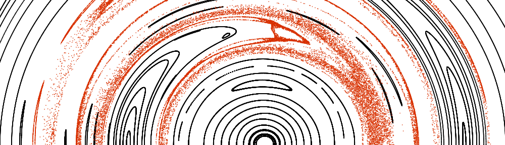
Although there are several ways by which one or more planets might destabilise other bodies, the one with the widest applicability is the overlap of mean motion resonances. These resonances occur when two bodies’ orbital periods are in a simple integer ratio, such as 2:1. From Kepler’s Law, , this occurs at a ratio of semi-major axes of around 1.6. So if one planet is located at 1AU, a planet at 1.6AU would be at the 2:1 resonance. Resonances with Neptune in the Kuiper Belt are shown schematically here:

Resonances in the Kuiper Belt. Note that the resonances become more closely spaced the closer they are to Neptune. Image Credit: Wikipedia

Now, although the actual period ratio only occurs at one specific semi-major axis ratio, the resonance also affects nearby orbits. The elements of these orbits oscillate, with a maximum amplitude of oscillation that depends on the mass of the planet and the particular resonance being considered. In particular, the more massive the planet, the more powerful the resonance, and the greater the range of semi-major axes affected by it. If a resonance acts alone on an orbit, the result is a regular oscillation of the orbital elements.

However, since the resonances have a width, and bunch up more closely the closer you are to the planet, there comes a point where the resonances overlap. When this happens, the evolution of an orbit becomes chaotic and unpredictable—crudely, instead of being confined to one resonance, you can imagine the particle being passed amongst many since their regions of oscillation overlap. This overlap of resonances driving chaotic behaviour was described by Chirikov (1979) and applied to the stability of orbits in the Solar System’s Asteroid Belt by Wisdom (1980).

It is useful to have a simple formula to give the boundary of the chaotic region for any planet mass. This Wisdom derived assuming low particle eccentricities, finding , where is the width of the cleared chaotic zone and is the ratio of planet mass to stellar mass. I.e., more massive planets clear out wider regions around their orbit, which is what one intuitively expects. This result is now used to estimate the mass of planets truncating debris discs, since if the planet and disc location are known, one can solve for .

In our previous paper, we had used the Wisdom result to estimate the amount of material that would destabilised as the star loses mass (this changes and so changes the width of the chaotic zone), and compared it to more accurate numerical results using both integrations of the full equations of motion, and a simpler numerical investigation using a dynamical map (described in Duncan, Quinn & Tremaine 1989). We considered a disc in which particles had moderate eccentricities, up to 0.1, since in our Solar System the Kuiper Belt bodies have eccentricities in this range. We found that the chaotic zone width increases with increasing eccentricity—this is also seen in Wisdom’s original paper, although Wisdom’s analytical result was only valid for low eccentricities. In our latest paper, we followed up these investigations, deriving a simple formula for the chaotic zone width at non-zero eccentricity.

In the next post, I’ll describe what exactly we did in our new paper, and the implications for the interactions of planets with planetesimal discs. Concisely, we found that if particles are on eccentric orbits, the width of the chaotic zone is no longer given by the Wisdom (1980) formula, and thus any attempt to estimate a planet mass in the way described above will give an erroneous result.